
Mathematical Insights#
[1]:
import matplotlib.pyplot as plt
import numpy as np
import pandas as pd
from optimask import OptiMask
from optimask.utils import generate_mar, plot
1. OptiMask API#
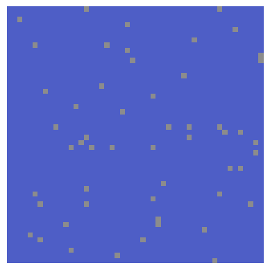
OptiMask is easy to use. It can be applied to NumPy arrays or pandas DataFrames, returning a subarray or subframe without NaN or the retained rows/columns. Since multiple optimizations are carried out starting from random states, a random_state parameter is provided for reproducibility.
[2]:
x = generate_mar(m=50, n=50, ratio=0.02)
plot(x)
[3]:
rows, cols = OptiMask(n_tries=50, random_state=0).solve(x)
len(rows), len(cols), np.any(np.isnan(x[rows][:, cols]))
[3]:
(34, 33, np.False_)
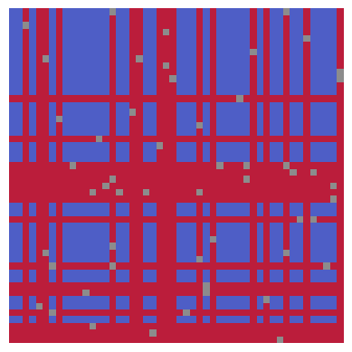
In red the removed rows and columns, in blue the remaining submatrix without NaN:
[4]:
plot(x, rows_to_keep=rows, cols_to_keep=cols)
OptiMask can directly return the submatrix:
[5]:
xt = OptiMask(random_state=0).solve(x, return_data=True)
xt.shape, np.any(np.isnan(xt))
[5]:
((30, 37), np.False_)
OptiMask offers a verbose mode to inspect the results of the intermediate optimizations:
[6]:
xt = OptiMask(random_state=0, verbose=True).solve(x, return_data=True)
xt.shape, np.any(np.isnan(xt))
        Trial 1 : submatrix of size 32x33 (1056 elements) found.
        Trial 2 : submatrix of size 28x36 (1008 elements) found.
        Trial 3 : submatrix of size 30x37 (1110 elements) found.
        Trial 4 : submatrix of size 28x38 (1064 elements) found.
        Trial 5 : submatrix of size 28x38 (1064 elements) found.
Result: the largest submatrix found is of size 30x37 (1110 elements) found.
[6]:
((30, 37), np.False_)
OptiMask provides a n_tries parameter, which enhances the probability of finding a better solution:
[7]:
%time xt = OptiMask(n_tries=35, random_state=0, verbose=True).solve(x, return_data=True)
xt.shape, np.any(np.isnan(xt))
CPU times: total: 125 ms
Wall time: 19.7 ms
        Trial 6 : submatrix of size 28x38 (1064 elements) found.
        Trial 7 : submatrix of size 33x33 (1089 elements) found.
        Trial 8 : submatrix of size 34x31 (1054 elements) found.
        Trial 9 : submatrix of size 32x34 (1088 elements) found.
        Trial 10 : submatrix of size 32x34 (1088 elements) found.
        Trial 11 : submatrix of size 32x31 (992 elements) found.
        Trial 12 : submatrix of size 28x38 (1064 elements) found.
        Trial 13 : submatrix of size 33x30 (990 elements) found.
        Trial 14 : submatrix of size 32x34 (1088 elements) found.
        Trial 15 : submatrix of size 32x33 (1056 elements) found.
        Trial 16 : submatrix of size 31x35 (1085 elements) found.
        Trial 17 : submatrix of size 32x34 (1088 elements) found.
        Trial 18 : submatrix of size 33x33 (1089 elements) found.
        Trial 19 : submatrix of size 32x32 (1024 elements) found.
        Trial 20 : submatrix of size 32x33 (1056 elements) found.
        Trial 21 : submatrix of size 32x33 (1056 elements) found.
        Trial 22 : submatrix of size 31x33 (1023 elements) found.
        Trial 23 : submatrix of size 29x37 (1073 elements) found.
        Trial 24 : submatrix of size 31x36 (1116 elements) found.
        Trial 25 : submatrix of size 31x32 (992 elements) found.
        Trial 26 : submatrix of size 32x32 (1024 elements) found.
        Trial 27 : submatrix of size 33x33 (1089 elements) found.
        Trial 28 : submatrix of size 32x33 (1056 elements) found.
        Trial 29 : submatrix of size 36x31 (1116 elements) found.
        Trial 30 : submatrix of size 28x38 (1064 elements) found.
        Trial 31 : submatrix of size 34x33 (1122 elements) found.
        Trial 32 : submatrix of size 33x32 (1056 elements) found.
        Trial 33 : submatrix of size 30x36 (1080 elements) found.
        Trial 34 : submatrix of size 33x33 (1089 elements) found.
        Trial 35 : submatrix of size 29x36 (1044 elements) found.
Result: the largest submatrix found is of size 34x33 (1122 elements) found.
[7]:
((34, 33), np.False_)
OptiMask can also handle pandas DataFrames:
[8]:
df = pd.DataFrame(x, columns=[f"feature {k}" for k in range(x.shape[1])])
df.sample(3)
[8]:
| feature 0 | feature 1 | feature 2 | feature 3 | feature 4 | feature 5 | feature 6 | feature 7 | feature 8 | feature 9 | ... | feature 40 | feature 41 | feature 42 | feature 43 | feature 44 | feature 45 | feature 46 | feature 47 | feature 48 | feature 49 | |
|---|---|---|---|---|---|---|---|---|---|---|---|---|---|---|---|---|---|---|---|---|---|
| 18 | 0.0 | 0.0 | 0.0 | 0.0 | 0.0 | 0.0 | 0.0 | 0.0 | 0.0 | 0.0 | ... | 0.0 | 0.0 | 0.0 | NaN | 0.0 | NaN | 0.0 | 0.0 | 0.0 | 0.0 |
| 47 | 0.0 | 0.0 | NaN | 0.0 | 0.0 | 0.0 | 0.0 | 0.0 | 0.0 | 0.0 | ... | 0.0 | 0.0 | 0.0 | 0.0 | 0.0 | 0.0 | 0.0 | 0.0 | 0.0 | 0.0 |
| 39 | 0.0 | 0.0 | 0.0 | 0.0 | 0.0 | 0.0 | 0.0 | 0.0 | 0.0 | 0.0 | ... | 0.0 | 0.0 | 0.0 | 0.0 | 0.0 | 0.0 | 0.0 | 0.0 | 0.0 | NaN |
3 rows × 50 columns
[9]:
df.info()
<class 'pandas.core.frame.DataFrame'>
RangeIndex: 50 entries, 0 to 49
Data columns (total 50 columns):
 #   Column      Non-Null Count  Dtype
---  ------      --------------  -----
 0   feature 0   50 non-null     float64
 1   feature 1   50 non-null     float64
 2   feature 2   49 non-null     float64
 3   feature 3   50 non-null     float64
 4   feature 4   49 non-null     float64
 5   feature 5   48 non-null     float64
 6   feature 6   48 non-null     float64
 7   feature 7   49 non-null     float64
 8   feature 8   50 non-null     float64
 9   feature 9   49 non-null     float64
 10  feature 10  50 non-null     float64
 11  feature 11  49 non-null     float64
 12  feature 12  48 non-null     float64
 13  feature 13  49 non-null     float64
 14  feature 14  49 non-null     float64
 15  feature 15  46 non-null     float64
 16  feature 16  49 non-null     float64
 17  feature 17  50 non-null     float64
 18  feature 18  49 non-null     float64
 19  feature 19  49 non-null     float64
 20  feature 20  49 non-null     float64
 21  feature 21  49 non-null     float64
 22  feature 22  49 non-null     float64
 23  feature 23  48 non-null     float64
 24  feature 24  49 non-null     float64
 25  feature 25  50 non-null     float64
 26  feature 26  49 non-null     float64
 27  feature 27  50 non-null     float64
 28  feature 28  47 non-null     float64
 29  feature 29  48 non-null     float64
 30  feature 30  49 non-null     float64
 31  feature 31  49 non-null     float64
 32  feature 32  50 non-null     float64
 33  feature 33  50 non-null     float64
 34  feature 34  49 non-null     float64
 35  feature 35  48 non-null     float64
 36  feature 36  49 non-null     float64
 37  feature 37  50 non-null     float64
 38  feature 38  49 non-null     float64
 39  feature 39  50 non-null     float64
 40  feature 40  49 non-null     float64
 41  feature 41  47 non-null     float64
 42  feature 42  49 non-null     float64
 43  feature 43  49 non-null     float64
 44  feature 44  49 non-null     float64
 45  feature 45  48 non-null     float64
 46  feature 46  50 non-null     float64
 47  feature 47  49 non-null     float64
 48  feature 48  48 non-null     float64
 49  feature 49  48 non-null     float64
dtypes: float64(50)
memory usage: 19.7 KB
[10]:
dft = OptiMask(n_tries=35).solve(df, return_data=True)
dft.info()
<class 'pandas.core.frame.DataFrame'>
Index: 33 entries, 2 to 48
Data columns (total 34 columns):
 #   Column      Non-Null Count  Dtype
---  ------      --------------  -----
 0   feature 0   33 non-null     float64
 1   feature 1   33 non-null     float64
 2   feature 3   33 non-null     float64
 3   feature 5   33 non-null     float64
 4   feature 6   33 non-null     float64
 5   feature 7   33 non-null     float64
 6   feature 8   33 non-null     float64
 7   feature 9   33 non-null     float64
 8   feature 10  33 non-null     float64
 9   feature 11  33 non-null     float64
 10  feature 14  33 non-null     float64
 11  feature 16  33 non-null     float64
 12  feature 17  33 non-null     float64
 13  feature 19  33 non-null     float64
 14  feature 20  33 non-null     float64
 15  feature 21  33 non-null     float64
 16  feature 25  33 non-null     float64
 17  feature 26  33 non-null     float64
 18  feature 27  33 non-null     float64
 19  feature 31  33 non-null     float64
 20  feature 32  33 non-null     float64
 21  feature 33  33 non-null     float64
 22  feature 35  33 non-null     float64
 23  feature 37  33 non-null     float64
 24  feature 39  33 non-null     float64
 25  feature 40  33 non-null     float64
 26  feature 41  33 non-null     float64
 27  feature 42  33 non-null     float64
 28  feature 43  33 non-null     float64
 29  feature 44  33 non-null     float64
 30  feature 45  33 non-null     float64
 31  feature 46  33 non-null     float64
 32  feature 47  33 non-null     float64
 33  feature 48  33 non-null     float64
dtypes: float64(34)
memory usage: 9.0 KB
[11]:
index, columns = OptiMask(n_tries=35).solve(df)
index, columns
[11]:
(Index([ 0,  1,  2,  3,  5,  6,  9, 10, 12, 14, 16, 17, 19, 20, 21, 23, 27, 28,
        30, 31, 32, 33, 35, 37, 38, 40, 41, 44, 45, 46, 47, 48, 49],
       dtype='int64'),
 Index(['feature 0', 'feature 1', 'feature 3', 'feature 5', 'feature 6',
        'feature 8', 'feature 9', 'feature 10', 'feature 11', 'feature 16',
        'feature 17', 'feature 18', 'feature 19', 'feature 20', 'feature 22',
        'feature 24', 'feature 25', 'feature 26', 'feature 27', 'feature 29',
        'feature 30', 'feature 31', 'feature 32', 'feature 33', 'feature 34',
        'feature 35', 'feature 36', 'feature 37', 'feature 39', 'feature 42',
        'feature 43', 'feature 45', 'feature 46', 'feature 47'],
       dtype='object'))
2. Understanding the problem at hand#
In the context of a matrix containing a lone NaN cell, the central challenge emerges: determining whether to eliminate the corresponding row or column. This decision is readily resolved by examining the matrix’s shape. Specifically, if the matrix has a greater number of rows than columns, the optimal approach involves removing the associated row. Conversely, when the matrix has more columns than rows, the most effective course of action is to eliminate the corresponding column:
[12]:
x = np.zeros((12, 5))
x[7, 1] = np.nan

plt.figure()
plt.subplot(1, 3, 1)
plot(x, show=False, title="original data")
plt.subplot(1, 3, 2)
plot(x, rows_to_remove=[7], show=False, title="remove row")
plt.subplot(1, 3, 3)
plot(x, cols_to_remove=[1], show=False, title="remove column")
plt.show()
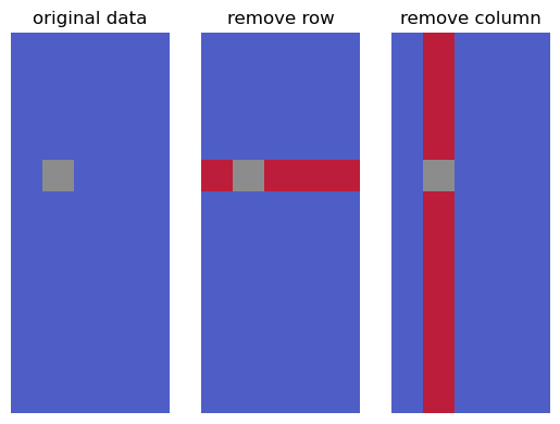
Eliminating the highlighted row yields the most extensive submatrix devoid of NaN. This solution remains optimal even when additional NaN values are present within the same row:
[13]:
x = np.zeros((12, 5))
x[7, [1, 3]] = np.nan

plt.figure()
plt.subplot(1, 3, 1)
plot(x, show=False, title="original data")
plt.subplot(1, 3, 2)
plot(x, rows_to_remove=[7], show=False, title="remove row")
plt.subplot(1, 3, 3)
plot(x, cols_to_remove=[1, 3], show=False, title="remove columns")
plt.show()
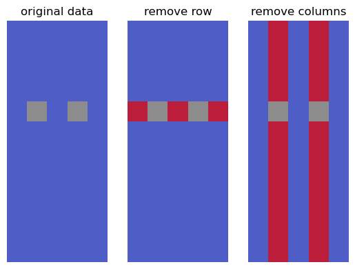
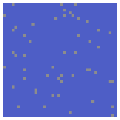
But what about more complex cases ?
[14]:
m, n = 40, 40
ratio = 0.03
x = generate_mar(m, n, ratio)

plot(x)
3. The Problem from an Optimization Perspective#
This problem can be formalized as a binary optimization problem in two ways.
3.1. Linear programming#
Source : this mathematica.stackexchange answer, posted by unlikely.
Given:
Matrix \(A\) of shape \(m \times n\) and elements \(a_{i,j}\)
The goal is to determine the values of variables \((i \in [1~..~m]\), \(j \in [1~..~n])\):
\(e_{i,j} \in \{0,1\}\) (1 if element \((i,j)\) should be removed, 0 otherwise)
\(r_i \in \{0,1\}\) (1 if row \(i\) should be removed, 0 otherwise)
\(c_j \in \{0,1\}\) (1 if column \(j\) should be removed, 0 otherwise)
Subject to:
\(e_{i,j} = 1\) for every \((i,j)\) such that \(a_{i,j}\) is a NaN
\(r_i + c_j \geq e_{i,j}\), meaning if \(e_{i,j} = 1\) then either \(r_i = 1\) or \(c_j = 1\), or both
\(e_{i,j} \geq r_i\), indicating if \(r_i = 1\) then \(e_{i,j}\) must be 1
\(e_{i,j} \geq c_j\), indicating if \(c_j = 1\) then \(e_{i,j}\) must be 1
The objective is to minimize the total number of deleted cells:
The optimal values of \(r_i\) and \(c_j\) provide us with the specific rows and columns to remove, ensuring that the remaining matrix is efficiently processed and devoid of NaN values. This problem can be solved in Python using the usual tools of linear programming, such as combining Pyomo with GLPK. Its disadvantage is being relatively expensive, as for an \(m \times n\) matrix, more than \(m \times n\) (binary) variables are used.
[15]:
from pyomo.environ import Binary, ConcreteModel, ConstraintList, Objective, SolverFactory, Var, minimize


def linear_programming(matrix):
    m, n = matrix.shape
    model = ConcreteModel()

    # Variables
    model.e = Var(range(1, m + 1), range(1, n + 1), within=Binary)
    model.r = Var(range(1, m + 1), within=Binary)
    model.c = Var(range(1, n + 1), within=Binary)

    # Objective
    model.obj = Objective(
        expr=sum(model.e[i, j] for i in range(1, m + 1) for j in range(1, n + 1)),
        sense=minimize,
    )

    # Constraints
    positions = [(i, j) for i in range(1, m + 1) for j in range(1, n + 1)]
    nan_positions = [(i, j) for (i, j) in positions if np.isnan(matrix[i - 1, j - 1])]

    model.nan_constraints = ConstraintList()
    for i, j in nan_positions:
        model.nan_constraints.add(model.e[i, j] == 1)

    model.other_constraints = ConstraintList()
    for i, j in positions:
        model.other_constraints.add(model.r[i] + model.c[j] >= model.e[i, j])
        model.other_constraints.add(model.e[i, j] >= model.r[i])
        model.other_constraints.add(model.e[i, j] >= model.c[j])

    # Solve the model
    solver = SolverFactory("glpk")
    solver.solve(model)

    # Extract the results
    rows_to_keep = [i - 1 for i in range(1, m + 1) if model.r[i].value == 0]
    cols_to_keep = [j - 1 for j in range(1, n + 1) if model.c[j].value == 0]

    return rows_to_keep, cols_to_keep


%time rows, cols = linear_programming(x)

plot(x, rows_to_keep=rows, cols_to_keep=cols)
print(
    f"The largest submatrix without NaN is of size {len(rows)}x{len(cols)} ({len(rows)*len(cols)} elements among {xt.size})"
)
CPU times: total: 281 ms
Wall time: 1min 15s
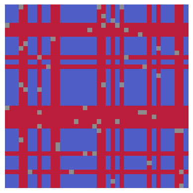
The largest submatrix without NaN is of size 28x27 (756 elements among 1122)
Although producing the optimal solution, this approach becomes intractable for large-sized matrices.
3.2. Quadratic Programming#
By employing the variables mentioned earlier, an alternate perspective of the problem involves maximizing
while considering: - \(r_i + c_j \ge 1\) for each \((i,j)\) where \(a_{i,j}\) is a NaN.
Although the number of variables is reduced, the optimization problem becomes more challenging.
4. OptiMask#
4.1. The algorithm#
OptiMask’s algorithm aims to identify the optimal set of rows and columns for removal, maximizing the size of the submatrix without NaN values. Notably, a formal proof of convergence for this algorithm is currently unavailable.
The algorithm iteratively computes permutations of rows and columns until a specific convergence criterion is met. This criterion relies on detecting a contiguous and well-ordered NaN frontier, similar to a Pareto efficiency frontier. Once identified, the problem simplifies to finding the largest contiguous rectangle, a computationally straightforward task. The stored permutations help pinpoint the rows and columns to be removed.
OptiMask’s algorithm is heuristic, introducing uncertainty compared to a linear programming approach. To increase the likelihood of an optimal solution, the algorithm undergoes multiple optimizations through repeated restarts with random permutations. The n_tries parameter controls the number of restarts, while the random_state parameter ensures reproducibility.
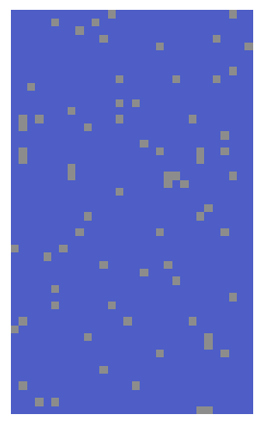
Let x represent the array with missing values to be processed:
[16]:
x = generate_mar(m=50, n=30, ratio=0.05)
plot(x)
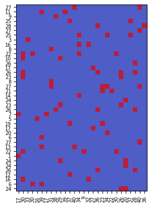
The first step is to isolate the rows and columns with at least one NaN value. We know that the rows or columns with zero NaN values will necessarily be part of the sought submatrix. Now we work with a boolean matrix, which is set to True at the NaN cells of the original data. We introduce hx and hy, representing the indices of the highest True in each column and the indices of the rightmost True in each row, respectively.
[17]:
def heights(x, axis=0):
    return (x.shape[axis] - np.argmax(np.flip(x, axis=axis), axis=axis)).astype(np.uint32)
[18]:
nan_rows, nan_cols = np.isnan(x).nonzero()
nan_rows, nan_cols = np.unique(nan_rows), np.unique(nan_cols)
xp = np.isnan(x[nan_rows][:, nan_cols])
hx, hy = heights(xp, axis=0), heights(xp, axis=1)
plot(xp, xticks=hx, yticks=hy)
The algorithm’s core involves computing a series of permutations with the objective of ordering hx and hy to establish a Pareto frontier of NaN. This implies that both hx and hy should exhibit a decreasing trend. Importantly, at each step, the algorithm performs a permutation to order hx, followed by a permutation to order hy, and then alternates back and forth between hx and hy until both sequences exhibit a decreasing order.
[19]:
hx, hy = heights(xp, axis=0).astype(np.uint32), heights(xp, axis=1).astype(np.uint32)
k = 0
while not (OptiMask.is_decreasing(hx) and OptiMask.is_decreasing(hy)):
    axis = k % 2
    p_step = np.argsort(-heights(xp, axis=axis))
    if axis == 0:
        xp = xp[:, p_step]
    if axis == 1:
        xp = xp[p_step]
    hx, hy = heights(xp, axis=0).astype(np.uint32), heights(xp, axis=1).astype(
        np.uint32
    )
    plot(xp, xticks=hx, yticks=hy, title=f"Iteration {k+1}")
    k += 1
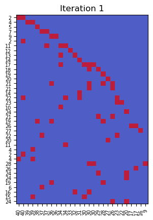
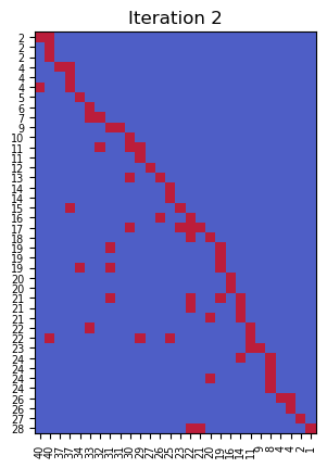
Then, we can now seek the largest contiguous rectangle starting from the upper right of the matrix (without forgetting the rows and columns without NaN, not displayed here). Since we have kept track of the successive permutations, both over rows and columns, the algorithm can return the rows and columns to remove (or keep).
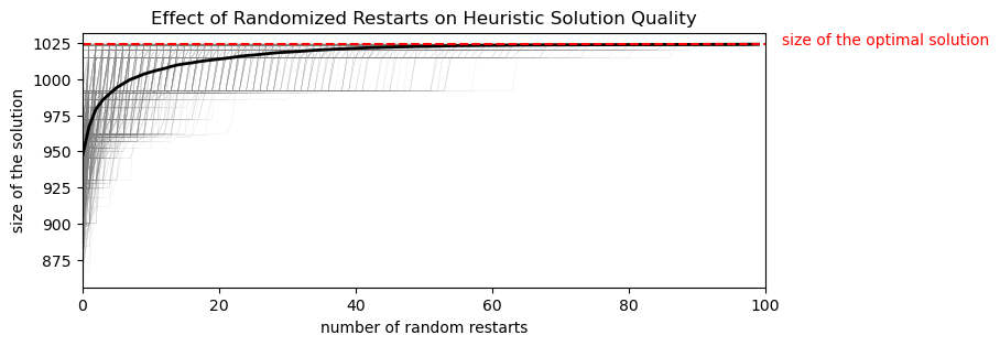
This computation is performed n_tries times over a copy of the matrix to process, where its rows and columns are each time randomly permuted. Each iteration results in a different NaN frontier and a different set of rows and columns to remove. After the n_tries computations, the set that leads to the largest submatrix without NaN is retained. Therefore, increasing n_tries leads to better results, and it may even reach the optimal one.
4.2. n_tries influence on the quality of the solution#
Given an mxn matrix with missing values occurring at a random frequency of ratio, how does increasing n_tries influence the size of the computed submatrix?
[20]:
def convergence_plot(m, n, ratio, n_tries, n_permutations=1000):
    def cummax(arr):
        return np.maximum.accumulate(arr)

    x = generate_mar(m, n, ratio)
    opt_rows, opt_cols = linear_programming(x)
    opt_size = len(opt_rows) * len(opt_cols)

    optimask = OptiMask(n_tries=1)

    ret = np.zeros(n_tries)
    for k in range(n_tries):
        rows, cols = optimask.solve(x)
        ret[k] = len(rows) * len(cols)

    ret_mean = np.zeros_like(ret, dtype=float)

    plt.figure(figsize=(8, 3))
    for _ in range(n_permutations):
        ret_iter = cummax(ret[np.random.permutation(len(ret))])
        plt.plot(ret_iter, c="grey", lw=0.05)
        ret_mean += ret_iter / n_permutations
    plt.plot(ret_mean, c="k", lw=2)
    plt.axhline(y=opt_size, c="r", linestyle="dashed")
    plt.xlabel("number of random restarts")
    plt.ylabel("size of the solution")
    plt.title("Effect of Randomized Restarts on Heuristic Solution Quality")
    plt.xlim(0, n_tries)
    plt.text(x=1.025 * n_tries, y=opt_size, s="size of the optimal solution", c="r")
    plt.show()
[21]:
convergence_plot(m=40, n=40, ratio=0.025, n_tries=100)
4.3. What about structured NaN patterns ?#
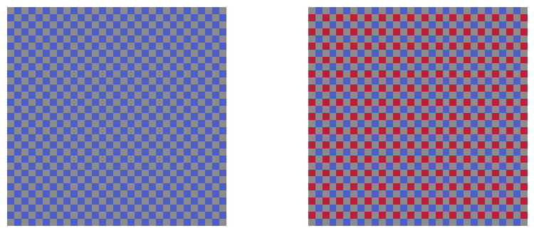
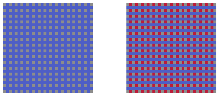
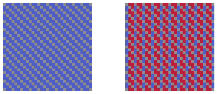
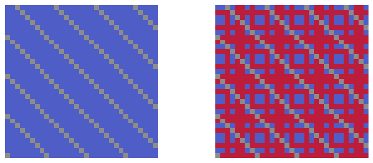
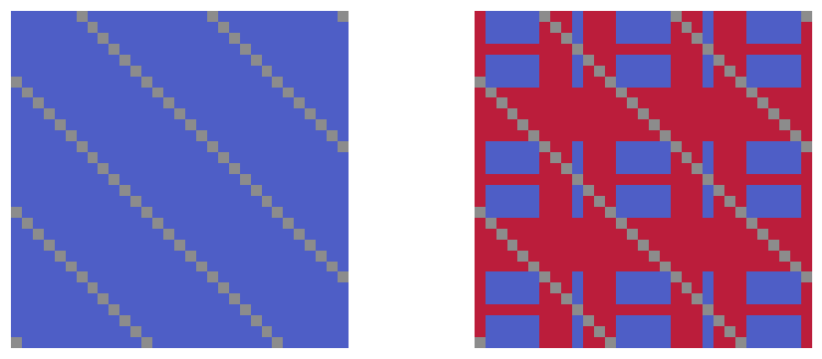
OptiMask is also efficient on structured NaN patterns (the largest submatrix found is in blue, the removed cells are in red):
[22]:
def solve_and_plot(x):
    rows, cols = OptiMask().solve(x)
    plt.figure(figsize=(10, 4))
    plt.subplot(1, 2, 1)
    plot(x, show=False)
    plt.subplot(1, 2, 2)
    plot(x, rows_to_keep=rows, cols_to_keep=cols)
    plt.show()
[23]:
n = 31
[24]:
x = np.zeros((n, n))
iy, ix = np.indices(x.shape)
x[np.mod(iy + ix, 2) == 0] = np.nan
solve_and_plot(x)
[25]:
x = np.zeros((n, n))
iy, ix = np.indices(x.shape)
x[(np.mod(ix, 2) == 0) & (np.mod(iy, 2) == 0)] = np.nan
solve_and_plot(x)
[26]:
x = np.zeros((n, n))
iy, ix = np.indices(x.shape)
x[np.mod(iy + ix, 3) == 0] = np.nan
solve_and_plot(x)
[27]:
x = np.zeros((n, n))
iy, ix = np.indices(x.shape)
x[np.mod(iy + ix, 8) == 0] = np.nan
solve_and_plot(x)
[28]:
x = np.zeros((n, n))
iy, ix = np.indices(x.shape)
x[np.mod(iy + ix, 12) == 0] = np.nan
solve_and_plot(x)
4.4. Dealing with large matrices#
OptiMask can efficiently handle large matrices within a reasonable amount of time. Its time complexity is proportional to the number of NaN cells, and the number n_tries.
[29]:
x = generate_mar(m=10_000, n=100, ratio=0.02)
%time rows, cols = OptiMask().solve(x)
np.isnan(x[rows][:, cols]).any()
CPU times: total: 0 ns
Wall time: 8.16 ms
[29]:
np.False_
[30]:
x = generate_mar(m=1_000, n=1_000, ratio=0.02)
%time rows, cols = OptiMask().solve(x)
np.isnan(x[rows][:, cols]).any()
CPU times: total: 0 ns
Wall time: 6.91 ms
[30]:
np.False_
[31]:
x = generate_mar(m=100_000, n=1_000, ratio=0.02)
%timeit rows, cols = OptiMask().solve(x)
215 ms ± 7.64 ms per loop (mean ± std. dev. of 7 runs, 1 loop each)
[32]:
x = generate_mar(m=1_000, n=100_000, ratio=0.02)
%timeit rows, cols = OptiMask().solve(x)
205 ms ± 4.35 ms per loop (mean ± std. dev. of 7 runs, 1 loop each)
[33]:
rows, cols = OptiMask(n_tries=25, verbose=True).solve(x)
        Trial 1 : submatrix of size 50x36409 (1820450 elements) found.
        Trial 2 : submatrix of size 50x36561 (1828050 elements) found.
        Trial 3 : submatrix of size 52x35089 (1824628 elements) found.
        Trial 4 : submatrix of size 48x38032 (1825536 elements) found.
        Trial 5 : submatrix of size 50x36497 (1824850 elements) found.
        Trial 6 : submatrix of size 51x35977 (1834827 elements) found.
        Trial 7 : submatrix of size 52x35273 (1834196 elements) found.
        Trial 8 : submatrix of size 49x37364 (1830836 elements) found.
        Trial 9 : submatrix of size 49x37102 (1817998 elements) found.
        Trial 10 : submatrix of size 51x35918 (1831818 elements) found.
        Trial 11 : submatrix of size 51x35543 (1812693 elements) found.
        Trial 12 : submatrix of size 50x36440 (1822000 elements) found.
        Trial 13 : submatrix of size 52x35405 (1841060 elements) found.
        Trial 14 : submatrix of size 50x36497 (1824850 elements) found.
        Trial 15 : submatrix of size 49x37421 (1833629 elements) found.
        Trial 16 : submatrix of size 49x37384 (1831816 elements) found.
        Trial 17 : submatrix of size 49x37359 (1830591 elements) found.
        Trial 18 : submatrix of size 50x36689 (1834450 elements) found.
        Trial 19 : submatrix of size 52x35216 (1831232 elements) found.
        Trial 20 : submatrix of size 50x36503 (1825150 elements) found.
        Trial 21 : submatrix of size 51x35725 (1821975 elements) found.
        Trial 22 : submatrix of size 50x36292 (1814600 elements) found.
        Trial 23 : submatrix of size 50x36502 (1825100 elements) found.
        Trial 24 : submatrix of size 49x37670 (1845830 elements) found.
        Trial 25 : submatrix of size 49x37248 (1825152 elements) found.
Result: the largest submatrix found is of size 49x37670 (1845830 elements) found.